Normalizing genomic signals

Abstract

This vignette covers the functions for normalizing genomic signals. Since this is illustrated with visualization, it is recommended that you read the bam2bw and multiRegionPlot vignettes first.

Introduction

epiwraps includes two ways of calculating normalization factors: either from the signal files (e.g. bam or bigwig files), which is the most robust way and enables all options, or from an EnrichmentSE object (see the multiRegionPlot vignette for an intro to such an object) or signal matrices. In both cases, the logic is the same: we estimate normalization factors (mostly single linear scaling factors, although some methods involve more complex normalization), and then apply them to signals that were extracted using signal2Matrix().

Applying normalization factors when generating the bigwig files

It is possible to also directly use computed normalization factors when creating bigwig files. By default, the bam2bw() function scales using library size, which can be disabled using scaling=FALSE. However, it is also possible to pass the scaling argument a manual scaling factor, as computed by the functions described here. In this vignette, however, we will focus on normalizing signal matrices.

Obtaining normalization factors for a set of signal files

The getNormFactors() function can be used to estimate normalization factors from either bam or bigwig files. The files cannot be mixed (bam/bigwig), however, and it is important to note that normalization factors calculated on bam files cannot be applied to data extracted from bigwig files, or vice versa, because the bigwig files are by default already normalized for library size. If needed, however, getNormFactors() can be used to apply the same method to both kind of files.

Normalization methods

Simple library size normalization, as done by bam2bw(), is not always appropriate. The main reasons are 1) that different samples/experiments can have a different signal-to-noise ratio, with the result that more sequencing is needed to obtain a similar coverage of enriched region; 2) that there might be global differences in the amount of the signal of interest (e.g. more or less binding, globally, in one cell type vs another); and 3) that there might be differences in technical biases, such as GC content. For these reasons, different normalization methods are needed according to circumstances and what assumptions seem reasonable. Here is an overview of the normalization methods currently implemented in epiwraps via the getNormFactors() function:

The ‘background’ or ‘SES’ normalization method (they are synonyms here) assumes that the background noise should on average be the same across experiments (Diaz et al., Stat Appl Gen et Mol Biol, 2012), an assumption that works well in practice and is robust to global differences in the amount of signal when there are not large differences in signal-to-noise ratio.
The ‘MAnorm’ approach ( Shao et al., Genome Biology 2012 ) assumes that regions that are commonly enriched (i.e. common peaks) in two experiments should on average have the same signal in the two experiments.
The ‘enriched’ approach assumes that enriched regions are on average similarly enriched across samples. Contrarily to ‘MAnorm’, these regions do not need to be in common across samples/experiments. This is not robust to global differences.
The ‘top’ approach assumes that the maximum enrichment (after some trimming) in peaks is the same across samples/experiments.
The ‘S3norm’ (Xiang et al., NAR 2020) and ‘2cLinear’ methods try to normalize both enrichment and background simultaneously. S3norm does this in a log-linear fashion (as in the publication), while ‘2cLinear’ does it on the original scale.

The normalization factors can be computed using getNormFactors() :

suppressPackageStartupMessages(library(epiwraps))
# we fetch the path to the example bigwig file:
bwf <- system.file("extdata/example_atac.bw", package="epiwraps")
# we'll just double it to create a fake multi-sample dataset:
bwfiles <- c(atac1=bwf, atac2=bwf)
nf <- getNormFactors(bwfiles, method="background")

## Comparing coverage in random regions...

nf

## atac1 atac2 
##     1     1

In this case, since the files are identical, the factors are both 1.

Some normalization methods addtionally require peaks as input, e.g.:

peaks <- system.file("extdata/example_peaks.bed", package="epiwraps")
nf <- getNormFactors(bwfiles, peaks = peaks, method="MAnorm")

## Comparing coverage in peaks...

(Note that MAnorm would normally require to have a list of peaks for each sample/experiment).

Once computed, the normalization factors can be applied to an EnrichmentSE object:

sm <- signal2Matrix(bwfiles, peaks, extend=1000L)

## Reading /home/runner/work/_temp/Library/epiwraps/extdata/example_atac.bw
## Reading /home/runner/work/_temp/Library/epiwraps/extdata/example_atac.bw

sm <- renormalizeSignalMatrices(sm, scaleFactors=nf)
sm

## class: EnrichmentSE 
## 2 tracks across 150 regions
## assays(2): normalized input
## rownames(150): 1:195054101-195054250 1:133522798-133523047 ...
##   1:22224734-22224983 1:90375438-90375787
## rowData names(0):
## colnames(2): atac1 atac2
## colData names(0):
## metadata(0):

The object now has a new assay, called normalized, which has been put in front and therefore will be used for most downstream usages unless the uses specifies otherwise. Note that for any downstream function it is however possible to specify which assay to use via the assay argument.

Obtaining normalization factors from the signal matrices themselves

It is also possible to normalize the signal matrices using factors derived from the matrices themselves, using the renormalizeSignalMatrices function. Note that this is provided as a ‘quick-and-dirty’ approach that does not have the robustness of proper estimation methods. Specifically, beyond providing manual scaling factors (e.g. computed using getNormFactors), the function includes two methods :

method="border" works on the assumption that the left/right borders of the matrices represent background signal which should be equal across samples. As such, it can be seen as an approximation of the aforementioned background normalization. However, it will work only if 1) the left/right borders of the matrices are sufficiently far from the signal (e.g. peaks) to be chiefly noise, and (as with the main background normalization method itself) 2) the signal-to-noise ratio is comparable across tracks/samples.
method="top" instead works on the assumption that the highest signal (after some eventual trimming of the extremes) should be the same across tracks/samples.

To illustrate these, we will first introduce some difference between our two tracks using arbitrary factors:

sm <- renormalizeSignalMatrices(sm, scaleFactors=c(1,4), toAssay="test")
plotEnrichedHeatmaps(sm, assay = "test")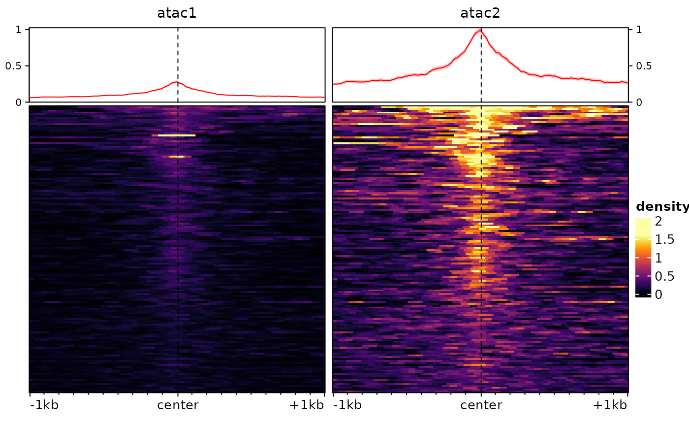

Then we can normalize:

sm <- renormalizeSignalMatrices(sm, method="top", fromAssay="test")
# again this adds an assay to the object, which will be automatically used when plotting:
plotEnrichedHeatmaps(sm)

## Using assay topNormalized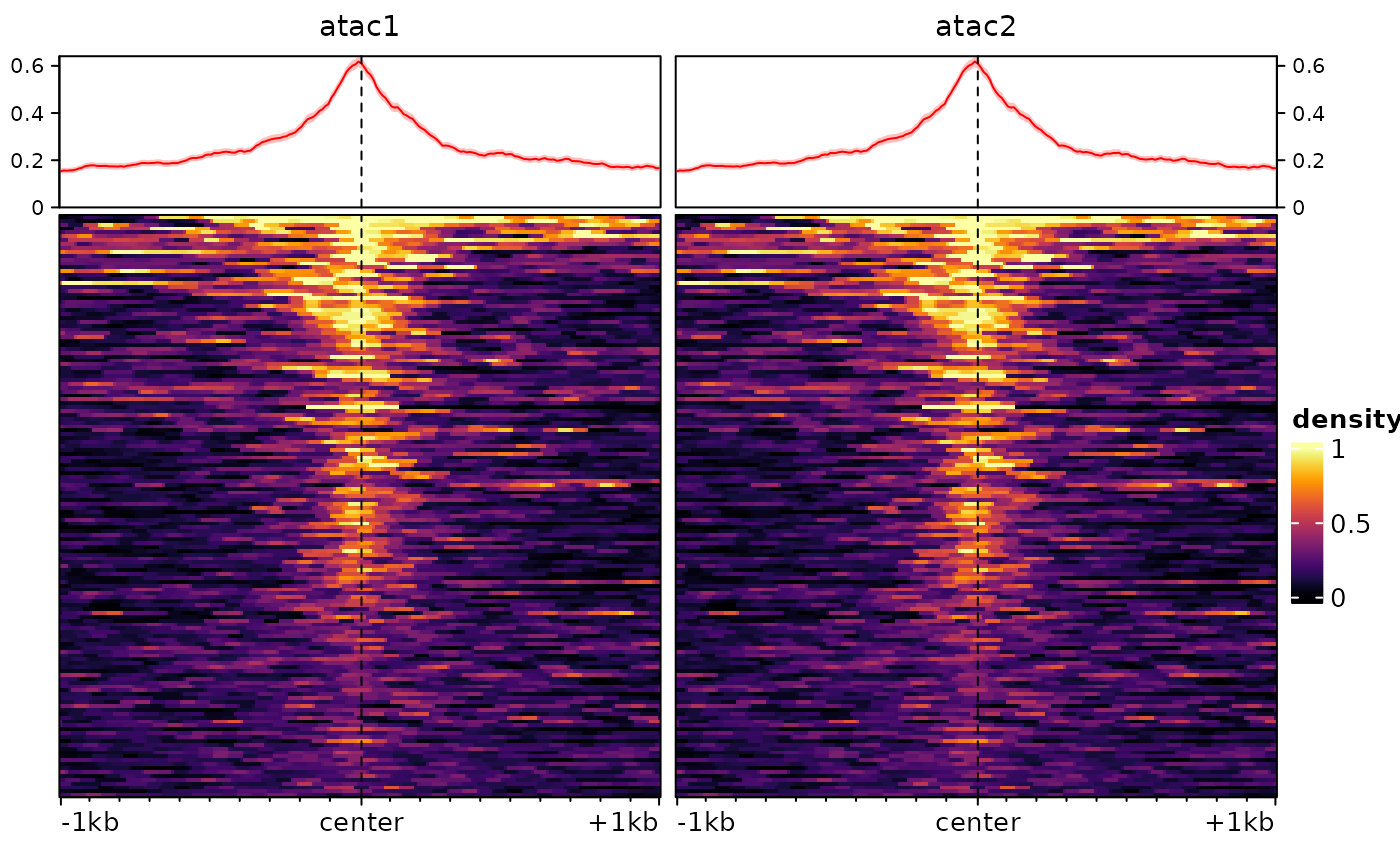

And we’ve recovered comparable signal across the two tracks/samples.

Session information

sessionInfo()